1. Why RAG is the most important pattern in enterprise AI

Every enterprise AI project eventually runs into the same wall.

You pick a frontier model — Claude, GPT-4o, Gemini. You build a prototype. It is impressive. Then someone asks it about your internal product catalog, your compliance policy from last quarter, your incident runbook from last week. The model either makes something up or admits it does not know.

This is not a model failure. It is an architectural gap.

LLMs are trained on public data up to a cutoff date. They have no knowledge of your enterprise's proprietary documents, internal systems, or anything that happened after their training ended. No matter how powerful the model, it cannot retrieve what it was never shown.

Retrieval-Augmented Generation (RAG) solves this by separating knowledge storage from language generation. Instead of baking knowledge into model weights — which is expensive, slow, and brittle — RAG retrieves the relevant knowledge at query time and injects it into the context window. The model reasons over what you give it, not just what it learned during training.

This is why RAG has become the dominant pattern in enterprise AI. It is not the most glamorous technique. But it is the one that makes AI systems actually useful in production environments where proprietary, current, and accurate information matters.

RAG does not make the model smarter. It makes the model better informed. The distinction matters architecturally — you are building a retrieval system as much as an AI system.

2. How RAG works — the architecture

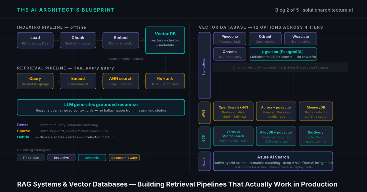
RAG has two distinct pipelines that run at different times. Understanding this separation is the first step to designing it correctly.

The indexing pipeline (runs once, or on a schedule)

This is the offline pipeline that prepares your knowledge base for retrieval. It runs when you add new documents, update existing ones, or refresh your data.

Step 1 — Load: Ingest your source documents. PDFs, Word files, web pages, database records, SharePoint, Confluence — anything that contains knowledge your system needs to access.

Step 2 — Chunk: Split documents into smaller pieces. A full 200-page product manual cannot fit in a context window alongside a query and a response. Chunking breaks it into retrievable units. How you chunk determines everything about what you can retrieve.

Step 3 — Embed: Convert each chunk into a vector using an embedding model. This vector captures the semantic meaning of the chunk in high-dimensional space. Chunks about "equipment maintenance" and "machine servicing" will produce similar vectors even if the exact words differ.

Step 4 — Store: Write each chunk and its vector into a vector database, along with metadata (source document, date, category, department — whatever filters you might need later).

The retrieval pipeline (runs on every query)

This is the live pipeline that runs when a user asks a question.

Step 1 — Embed the query: Convert the user's question into a vector using the same embedding model used during indexing. This is critical — mismatched embedding models between indexing and retrieval produce garbage results.

Step 2 — Search: Query the vector database for the chunks whose vectors are most similar to the query vector. This is approximate nearest neighbour (ANN) search.

Step 3 — Re-rank (optional but recommended): Run the top-K retrieved chunks through a re-ranker model to reorder them by true relevance. This catches cases where semantic similarity did not perfectly align with actual relevance.

Step 4 — Inject into context: Assemble the retrieved chunks, the system prompt, and the user's query into the context window. This is context assembly — a design responsibility most teams underestimate.

Step 5 — Generate: Send the assembled context to the LLM. The model now has the relevant knowledge in front of it and generates a grounded response.

→ INSERT DIAGRAM 1: RAG Architecture (HTML card) here

3. Chunking strategies — the most underrated decision in RAG

If you get chunking wrong, nothing downstream can save you. A retrieval system can only return what was indexed well. If your chunks mix topics, cut sentences mid-thought, or are sized poorly for your embedding model, your retrieval quality will silently suffer — and the model will produce confidently wrong answers.

Most teams treat chunking as a default setting. It is one of the most important architectural decisions in your entire RAG stack.

Fixed-size chunking

Split every document into chunks of N characters or N tokens, with an overlap of M tokens between consecutive chunks. Simple to implement, predictable, and utterly naive.

The problem: A fixed-size split has no awareness of document structure. It will happily split a sentence in half, cut a table across two chunks, or blend the end of one section with the beginning of another. The overlap helps reduce boundary losses but does not solve the fundamental problem.

When to use it: Never in production. Acceptable only for a quick prototype to validate the rest of your pipeline.

Recursive character splitting

Split on a hierarchy of separators — paragraphs first, then sentences, then words — until each chunk falls within your target size. This is the default in LangChain and LlamaIndex for good reason.

The advantage: It respects natural language boundaries more than fixed-size splitting. Paragraphs stay together. Sentences are not cut mid-thought.

The limitation: It still has no awareness of document semantics — it does not know that a heading on page 3 belongs to the section that follows it, or that a table row without its header is meaningless.

When to use it: The safe default for most text-based documents when you do not have time to implement something more sophisticated.

Semantic chunking

Instead of splitting by size or separator, split by meaning. Compute embeddings for each sentence, then group consecutive sentences whose embeddings are similar into a single chunk. Split when the semantic similarity drops — that is, when the topic shifts.

The advantage: Chunks represent coherent ideas rather than arbitrary text windows. Retrieval quality improves significantly because each chunk is about one thing.

The trade-off: More expensive to compute (every sentence needs an embedding during indexing). Chunk sizes become variable, which complicates downstream processing.

When to use it: For high-value knowledge bases where retrieval quality justifies the indexing cost. SOPs, compliance documents, technical manuals.

Document-aware chunking

Parse the document structure explicitly — headings, subheadings, tables, lists, code blocks — and use that structure to define chunk boundaries. A Markdown document with H2 headings becomes a set of chunks, one per section. A PDF with a clear table of contents maps naturally to chapter-level chunks.

The advantage: Context integrity is preserved. A chunk about "Equipment Calibration" contains everything under that heading, not a random 512-token window that might start mid-procedure.

The trade-off: Requires document parsing that understands structure. PDFs are notoriously inconsistent. Scanned documents need OCR first.

When to use it: Whenever your source documents have clear structure — technical documentation, policy manuals, product catalogs with defined sections.

Chunk size and overlap — the trade-off

Smaller chunks (128–256 tokens) retrieve more precisely but lose context. A single sentence about "the 240V breaker requirement" is highly specific but lacks the surrounding context that explains why it matters.

Larger chunks (512–1024 tokens) preserve more context but match less precisely. A 1000-token chunk about equipment installation might be retrieved for a query about voltage requirements — but most of its content is irrelevant.

The emerging best practice is parent-child chunking: index small chunks for precise retrieval, but return the larger parent chunk to the model for context. You get the precision of small chunks and the context of large ones.

Overlap (typically 10–20% of chunk size) ensures that information near chunk boundaries is captured in at least one chunk. Too little overlap loses boundary content; too much bloats your index and creates redundant retrievals.

The right chunk size is determined by your documents, your embedding model's optimal input length, and your query patterns. There is no universal answer — but 512 tokens with 10% overlap and recursive splitting is a reasonable starting point for most enterprise use cases.

4. Embeddings — turning meaning into vectors

The embedding model is the lens through which your entire knowledge base is interpreted. Every chunk you index is converted into a vector by this model, and every query is converted by the same model at retrieval time. The quality of those vectors determines the ceiling of your retrieval quality — no reranker or retrieval strategy can recover what a poor embedding model lost.

Choosing an embedding model

OpenAI text-embedding-3-large — strong general-purpose performance, 3072 dimensions (can be reduced), excellent for English enterprise content. The default choice if you are already using OpenAI's API.

Cohere Embed v3 — competitive with OpenAI, with a strong advantage: native support for specifying whether you are embedding a document or a query. This input-type awareness meaningfully improves retrieval precision. Also strong for multilingual use cases.

BGE (BAAI General Embedding) — the leading open-source embedding model family. BGE-M3 in particular supports dense, sparse, and multi-vector retrieval in a single model. Strong performance at zero API cost — the right choice for self-hosted or cost-sensitive deployments.

E5 (Microsoft) — another strong open-source option, particularly well-suited for tasks framed as question-answer pairs, which aligns well with RAG retrieval patterns.

Embedding dimensions and trade-offs

Higher dimensions capture more semantic nuance but cost more to store and search. A 1536-dimension embedding requires roughly 6KB per chunk. At one million chunks, that is 6GB of vector storage before indexes.

OpenAI's text-embedding-3 models support dimension reduction via Matryoshka Representation Learning — you can truncate to 256 or 512 dimensions with modest quality loss and significant storage savings. For cost-sensitive deployments at scale, this trade-off is often worth it.

The cardinal rule: same model for indexing and retrieval

Never embed your documents with one model and your queries with another. The vector spaces are incompatible — a vector from model A and a vector from model B are not measuring distance in the same space. This is one of the most common and catastrophic mistakes in RAG implementations.

If you switch embedding models, you must re-index your entire knowledge base.

Multimodal embeddings

If your knowledge base includes product images, diagrams, scanned tables, or charts, text-only embeddings cannot represent them. Multimodal embedding models — such as OpenAI's CLIP-based models or Google's multimodal embeddings on Vertex AI — embed both text and images into the same vector space, enabling retrieval across modalities.

For retail use cases with product imagery, or QSR operations with equipment diagrams, multimodal embeddings are worth evaluating once your text RAG pipeline is stable.

5. Vector databases — the storage layer for semantic search

A vector database is purpose-built for one operation that traditional databases handle poorly: finding the K most similar vectors to a query vector across millions or billions of stored vectors, in milliseconds.

Traditional SQL databases can store vectors as arrays. But running a similarity search across 10 million rows with a full table scan is too slow for real-time retrieval. Vector databases solve this with Approximate Nearest Neighbour (ANN) indexes — data structures like HNSW (Hierarchical Navigable Small World) that trade a small amount of recall accuracy for massive search speed improvements.

The choice of vector database is one of the most consequential infrastructure decisions in your RAG architecture. Here is a complete comparison across the four tiers that matter for enterprise architects.

When a dedicated vector database is overkill

Before committing to a new piece of infrastructure, ask: how many vectors do you actually have?

For most enterprise RAG pilots and early production deployments — under 500K chunks — pgvector on PostgreSQL is genuinely sufficient. If your team already operates Postgres, adding the pgvector extension takes minutes. You get vector similarity search, metadata filtering, and full SQL expressiveness in one system you already know how to run, monitor, and backup.

The calculus changes when you need:

• Billions of vectors at sub-10ms latency
• Multi-tenancy across hundreds of customers
• Native hybrid search without building it yourself
• Geo-distributed search with low-latency global access

At that point, a dedicated vector database earns its operational overhead.

6. Retrieval strategies — beyond basic similarity search

Most RAG tutorials show you the simplest retrieval strategy: embed the query, find the top-5 similar chunks, inject them into the prompt. This works in demos. It underperforms in production.

Here is the full toolkit.

Dense retrieval

Pure vector similarity search. Embed the query, compute cosine similarity or dot product against all indexed vectors, return the top-K results. Fast, scalable, and semantically powerful.

The weakness: Dense retrieval struggles with exact keyword matches. If a user asks about "SKU-49271-B" and that exact string is in your documents, dense retrieval may miss it because the embedding captures semantic meaning, not exact character sequences. Product codes, regulation numbers, and proper nouns are all vulnerable.

Sparse retrieval — BM25

Traditional keyword-based search using term frequency and inverse document frequency. BM25 does not understand meaning but is exceptionally good at exact matching. It will find "SKU-49271-B" every time.

The weakness: It has no semantic understanding. A query for "equipment maintenance" will not match a document that uses "machine servicing" throughout.

Hybrid retrieval — the production default

Combine dense and sparse retrieval. Run both searches, then merge the result sets using Reciprocal Rank Fusion (RRF) or a weighted score combination. Each strategy compensates for the other's weakness.

In practice, hybrid retrieval outperforms either approach alone on almost every enterprise knowledge base. It is the default you should build toward from day one, even if you start with dense-only for simplicity.

Weaviate, Azure AI Search, and Elasticsearch all support hybrid retrieval natively. Qdrant and Pinecone support it via separate sparse vector storage.

Re-ranking

After retrieving the top-K candidates (typically 20–50), run them through a cross-encoder re-ranker that scores each chunk against the query jointly — rather than independently as in embedding-based retrieval.

Cross-encoders are slower than embedding models (they cannot be pre-computed) but significantly more accurate at ranking relevance. Models like Cohere Rerank or open-source BGE-Reranker are purpose-built for this.

The pattern: retrieve broadly (top-50), then re-rank and truncate (top-5). You get the recall of a wide retrieval with the precision of a careful reranker.

Metadata filtering

Before running vector search, filter your candidate set by metadata. If a QSR manager in Texas asks about equipment compliance, filter first to documents tagged region: US-South and category: compliance — then run vector search over that subset.

This dramatically improves precision and reduces the chance of retrieving irrelevant content from other regions, departments, or time periods.

Parent-child retrieval

Index small child chunks (128–256 tokens) for precise matching. When a child chunk is retrieved, return its larger parent chunk (512–1024 tokens) to the LLM for context.

This solves the chunk size trade-off directly: you get the retrieval precision of small chunks and the contextual richness of large ones.

7. Retrieval evaluation — how do you know if it's working?

Most teams skip this step entirely. They build a RAG pipeline, ask it a few questions, decide it "seems good," and ship it. Six weeks later, users are complaining that the system gives wrong answers — and the team has no idea whether the problem is retrieval or generation.

Evaluation is not optional. It is the only way to know whether your RAG system is improving or degrading as you make changes.

Key metrics — explained plainly

Recall@K — of all the relevant chunks that exist in your knowledge base for a given query, what fraction did your retrieval return in the top-K results? A Recall@5 of 0.8 means 80% of the time, the right chunk was in the top 5 results. This is the primary metric for retrieval quality.

Mean Reciprocal Rank (MRR) — how high up in the result list did the first relevant chunk appear? A result ranked first scores 1.0; ranked second scores 0.5; ranked third scores 0.33. Higher MRR means relevant content appears closer to the top of the retrieval list, which matters when you truncate to top-3 or top-5 for the context window.

Normalized Discounted Cumulative Gain (NDCG) — a more nuanced metric that accounts for the full ordering of results, giving higher weight to relevant documents appearing earlier. Useful when you have graded relevance (some chunks are more relevant than others, not just relevant/not relevant).

The Ragas framework

Ragas is an open-source framework specifically designed for RAG evaluation. It provides automated metrics across four dimensions:

• Faithfulness — does the generated answer stick to the retrieved context, or does it hallucinate beyond it?
• Answer relevancy — does the answer actually address the question asked?
• Context precision — of the chunks retrieved, what fraction were actually relevant?
• Context recall — was all the information needed to answer the question present in the retrieved chunks?

Ragas uses an LLM judge to compute these metrics automatically, which makes it practical to run at scale without manual annotation.

Building a golden dataset

Automated metrics require a ground truth dataset — a set of questions paired with the correct source chunks and correct answers for your specific domain.

Building this is effort upfront but pays for itself immediately. Without a golden dataset, you cannot measure whether a chunking change improved retrieval, whether switching embedding models helped, or whether adding a reranker was worth it.

For QSR or retail use cases, a 100–200 question golden dataset covering your most common query types is a reasonable starting point. Have subject matter experts validate the correct source chunks for each question.

Diagnosing failures: retrieval vs. generation

When your RAG system gives a wrong answer, there are only two possible causes:

Retrieval failure — the right information was never retrieved. The model had nothing to work with and either hallucinated or said it did not know. Diagnose by checking whether the correct chunk appears in the retrieved context for the failed query.

Generation failure — the right information was retrieved, but the model failed to use it correctly. It ignored the relevant chunk, misread a number, or hallucinated despite having the right context. Diagnose by manually inspecting the retrieved chunks and checking whether a human could answer the query from them.

These two failure modes require completely different fixes. Confusing them is one of the most expensive mistakes in RAG development.

8. Advanced RAG patterns

Once your baseline RAG pipeline is stable and measured, these patterns address specific limitations.

HyDE — Hypothetical Document Embeddings

Instead of embedding the raw query, ask the LLM to generate a hypothetical answer to the query first — even if that answer might be wrong. Then embed that hypothetical answer and use it for retrieval.

Why it works: A hypothetical answer looks more like a real document than a question does. Queries and documents live in slightly different parts of the embedding space. HyDE bridges that gap by generating something that resembles the target document.

Best for: Domains where queries are very short or vague and documents are long and detailed. Works well for technical documentation retrieval.

Query expansion and rewriting

Rewrite the user's query before retrieval to improve matching. Techniques include:

• Query expansion: generate multiple versions of the query covering different phrasings, then retrieve for each and merge results
• Query decomposition: break a complex multi-part query into sub-queries, retrieve for each, then synthesise
• Step-back prompting: rewrite the query at a higher level of abstraction before retrieval

Agentic RAG

Instead of a fixed retrieve-then-generate pipeline, let an agent decide when to retrieve, what to retrieve, and whether to retrieve again based on the initial results.

An agentic RAG system might: retrieve once, evaluate whether the results are sufficient, formulate a more specific follow-up query, retrieve again, then synthesise across multiple retrieval rounds. This is significantly more powerful for complex multi-step queries but requires careful latency management.

We cover agentic patterns in depth in Blog 3.

GraphRAG

Traditional RAG retrieves isolated chunks. GraphRAG builds a knowledge graph over your documents — entities, relationships, and communities — and retrieves over that graph structure rather than raw text chunks.

The advantage: GraphRAG can answer questions that require connecting information across multiple documents — "What are all the compliance requirements that affect our Texas locations?" — which chunk-based retrieval struggles with.

The trade-off: Significantly more complex to build and maintain. Best suited for knowledge bases with rich entity relationships (regulatory documents, product dependency graphs, organisational knowledge).

Microsoft's open-source GraphRAG implementation is the most mature option currently available.

9. Real-world application — Retail & QSR use cases

QSR Operations Copilot

A quick-service restaurant group wants their store managers to be able to query a system for operational guidance — food safety procedures, equipment troubleshooting, shift scheduling rules, compliance requirements.

RAG architecture decisions:

• Source documents: SOPs (PDFs), equipment manuals (PDFs + images), compliance docs (structured), HR policies (Word)
• Chunking strategy: Document-aware chunking — SOPs have clear section structure; respect it. Equipment manuals need parent-child chunking — retrieve at the procedure level, return the full procedure section
• Embedding model: BGE-M3 (open source, self-hosted) — operational data stays on-premise; no API calls for embedding
• Vector DB: Qdrant (self-hosted) — best performance-per-cost, runs on the same on-premise infrastructure as the LLM
• Retrieval strategy: Hybrid (dense + BM25) — equipment codes and regulation numbers need exact matching; procedure descriptions need semantic search
• Metadata filtering: Filter by store_region, equipment_type, and document_category before vector search
• Evaluation: Golden dataset of 150 operational queries validated by the operations team; Ragas for ongoing automated evaluation

Architecture Knowledge Assistant

An enterprise architecture team wants a system that can answer questions about internal architecture decisions — ADRs (Architecture Decision Records), runbooks, system diagrams, past incident reports.

RAG architecture decisions:

• Source documents: Confluence pages, ADRs (Markdown), runbooks (Markdown), incident reports (structured JSON + text)
• Chunking strategy: Semantic chunking — ADRs have variable structure; semantic splitting preserves decision context better than fixed splitting
• Embedding model: OpenAI text-embedding-3-large — cloud-hosted, internal architecture docs are not sensitive enough to require on-premise embedding
• Vector DB: Azure AI Search — the architecture team is already Azure-native; no new infrastructure, deep integration with existing Azure DevOps and SharePoint
• Retrieval strategy: Hybrid with re-ranking (Cohere Rerank) — architecture queries often involve specific system names and version numbers (needs BM25) plus conceptual similarity (needs dense)
• Metadata filtering: Filter by system_domain, document_type, and date_range — architecture decisions from 3 years ago may be superseded
• Evaluation: 100-question golden dataset covering common architecture queries; monthly re-evaluation as new ADRs are added

The same RAG pattern — index, retrieve, generate — produces completely different infrastructure choices depending on data sensitivity, existing cloud infrastructure, query patterns, and scale requirements.

Key takeaways

1. RAG separates knowledge from reasoning. The model reasons; your retrieval system provides the knowledge. Design both pipelines deliberately.
2. Chunking is the highest-leverage decision in your RAG stack. Invest time here before optimising anything else.
3. Same embedding model for indexing and retrieval. Always. No exceptions.
4. Hybrid retrieval is the production default. Dense search alone misses exact matches. Sparse search alone misses semantics. Combine them.
5. Measure retrieval separately from generation. Recall@K tells you whether the right chunk was found. Ragas tells you whether the model used it correctly. Confusing these two failure modes wastes months.
6. Vector DB choice follows your infrastructure. If you are AWS-native, evaluate OpenSearch and Aurora first. If you are on GCP, start with Vertex AI Vector Search or AlloyDB. Do not introduce new infrastructure for its own sake.
7. pgvector is often enough. For under 500K chunks, do not over-engineer the storage layer.
8. Advanced patterns (HyDE, GraphRAG, Agentic RAG) solve specific problems. Build a baseline first, measure it, then reach for advanced patterns for the specific failures you observe.

What's next

In Blog 3 — Agentic AI: Agents, MCP & Multi-Agent Systems, we move from retrieval to action. Agents do not just answer questions — they plan, use tools, call APIs, and coordinate with other agents to complete complex multi-step tasks. This is where enterprise AI gets genuinely transformative.

Follow along at solutionarchitecture.ai or subscribe below to get notified when Blog 3 drops.

— Firdous | Enterprise AI Architect | Designing Intelligent Systems for the AI-First Enterprise